If you are a current student, please Log In for full access to the web site.
Note that this link will take you to an external site (https://shimmer.csail.mit.edu) to authenticate, and then you will be redirected back to this page.
Error on line 7 of Python tag (line 8 of source):
    kerberos = cs_user_info['username']

KeyError: 'username'
In the next series of exercises we're going to learn how to think about and write a simple physics simulator to make a "rolling ball" on our LCD.
The result will be a system that looks like the following:
1) Physics
We're going to represent a ball on our LCD using the tft.fillCircle and/or tft.drawCircle functions that you may have already started messing with in Lab 01A. We'll then update its drawn position many times per second to make it look like it is moving. However, we want to make sure that it looks "real" so we need to build a simple physics engine and to do that we need to come up with a physics-based model that is code-compatible in order to code up this ball's motion and behavior. The first part of this is coming up with a consistent way of thinking about our coordinate space:
1.1) Frame of Reference
Generally when doing graphics, the origin (0,0) is in the top left of the screen with positive X pointing right and positive Y pointing downward. We'll follow that convention here so your screen has a coordinate field like the following: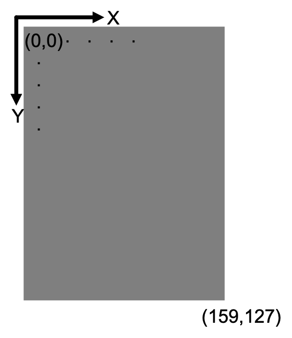
tft.setRotation(2); has been asserted!
We'll be simulating a moving ball so we'll need to also maintain consistency with this coordinate system when calculating the ball's acceleration, velocity, and position. For example, the ball's velocity vectors will be defined as following:

As you can see, positive y velocity is defined as down-pointing and positive x velocity defined as right-pointing.
2) Code and Modeling
To get us started, download the skeleton code file for our ball simulator HERE. We also have it printed out below for reference. Take a few minutes to read through it and start to digest it. There is a lot to take in.
#include <TFT_eSPI.h> // Graphics and font library for ST7735 driver chip
#include <SPI.h> //Used in support of TFT Display
#include <string.h>  //used for some string handling and processing.

TFT_eSPI tft = TFT_eSPI();  // Invoke library, pins defined in User_Setup.h

#define BACKGROUND TFT_GREEN
#define BALL_COLOR TFT_BLUE

const int DT = 40; //milliseconds
const int EXCITEMENT = 10000; //how much force to apply to ball
const uint8_t BUTTON_PIN = 16; //CHANGE YOUR WIRING TO PIN 16!!! (FROM 19)

uint32_t primary_timer; //main loop timer

//state variables:
float x_pos = 64; //x position
float y_pos = 32; //y position
float x_vel = 0; //x velocity
float y_vel = 0; //y velocity
float x_accel = 0; //x acceleration
float y_accel = 0; //y acceleration

//physics constants:
const float MASS = 1; //for starters
const int RADIUS = 5; //radius of ball
const float K_FRICTION = 0.15;  //friction coefficient
const float K_SPRING = 0.9;  //spring coefficient

//boundary constants:
const int LEFT_LIMIT = RADIUS; //left side of screen limit
const int RIGHT_LIMIT = 127-RADIUS; //right side of screen limit
const int TOP_LIMIT = RADIUS; //top of screen limit
const int BOTTOM_LIMIT = 159-RADIUS; //bottom of screen limit

bool pushed_last_time; //for finding change of button (using bool type...same as uint8_t)

//will eventually replace with your improved step function!
void step(float x_force=0, float y_force=0 ){
  //update acceleration (from f=ma)
  x_accel = x_force/MASS;
  y_accel = y_force/MASS;
  //integrate to get velocity from current acceleration
  x_vel = x_vel + 0.001*DT*x_accel; //integrate, 0.001 is conversion from milliseconds to seconds
  y_vel = y_vel + 0.001*DT*y_accel; //integrate!!
  //
  moveBall(); //you'll write this from scratch!
}

void moveBall(){
  //your code here
}


void setup() {
  Serial.begin(115200); //for debugging if needed.
  pinMode(BUTTON_PIN,INPUT_PULLUP);
  tft.init();
  tft.setRotation(2);
  tft.setTextSize(1);
  tft.fillScreen(BACKGROUND);
  randomSeed(analogRead(0));  //initialize random numbers
  step(random(-EXCITEMENT,EXCITEMENT),random(-EXCITEMENT,EXCITEMENT)); //apply initial force to lower right
  pushed_last_time = false;
  primary_timer = millis();
}

void loop() {
  //draw circle in previous location of ball in color background (redraws minimal num of pixels, therefore is quick!)
  tft.fillCircle(x_pos,y_pos,RADIUS,BACKGROUND);
  //if button pushed *just* pushed down, inject random force into system
  //else, just run out naturally
  if (!digitalRead(BUTTON_PIN)){ //if pushed
    if(!pushed_last_time){ //if not previously pushed
      pushed_last_time = true;
      step(random(-EXCITEMENT,EXCITEMENT),random(-EXCITEMENT,EXCITEMENT)); //apply initial force to lower right
    }else{
      step();
    }
  }else{ //else not pushed
    pushed_last_time = false; //mark that we were not pushed
    step(); //step as usual
  }
  tft.fillCircle(x_pos,y_pos,RADIUS,BALL_COLOR); //draw new ball location

  while (millis()-primary_timer < DT); //wait for primary timer to increment
  primary_timer = millis();
}
The basic flow of this piece of code is:
- Check if there are any forces applied to the ball. In this code, we use button pushes to stimulate the ball. Upon pushing your button (hooked up to IO pin 16 **which is different than what we've been using1, so let's not use it..), a random force is applied to the ball, the magnitude of which is dictated by the
EXCITEMENTvariable. - Calculate acceleration if any forces are applied, and update velocity accordingly (integrate). This is done within the
stepfunction. - Update position based on current position and velocity. This is not yet implemented, but will be done within the
moveBallfunction. - draw new position
- wait until next time step
In this system, forces can only be applied to the ball through the step function. If you look at how that is declared and defined in the code you'll notice the two input arguments are set =0. This is a way to make the arguments take on a default value if they are not specified. As a result if we wanted to apply a force of 1 and 3 Newtons in the x and y dimensions, respectively you could do:
step(1,3)
and if you just wanted to let the ball run (and apply no force) you would just do:
step()
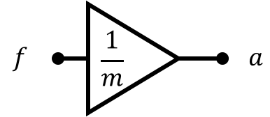
Let's look a bit more into what step is doing We can make our life a bit easier by assuming like we should have learned in 8.01 or AP Physics or whatever you took that we can handle each axis of motion separately. We first take in the force applied to the ball and divide it by the mass we've assigned (for simplicity it is 1 here, but feel free to change it later). Diagramatically we're doing the following, which is coming right from f = ma from 8.01.
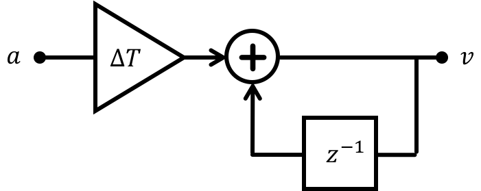
Once we've determined our acceleration in a given axis we will then integrate it to determine our velocity for that axis. 8.01 tells us that assuming we're starting from rest:
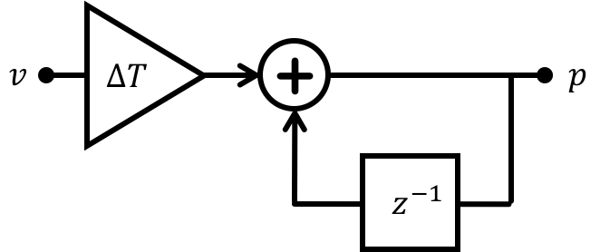
Finally we'll determine our position in each axis by integrating a second time:
2.1) States of Our System
When all put together, each dimension of freedom that our ball has is made up of three states represented by the red boxes below: acceleration, velocity, and position. These six values uniquely describe the state of a ball at each time step and are needed to fully describe its operation.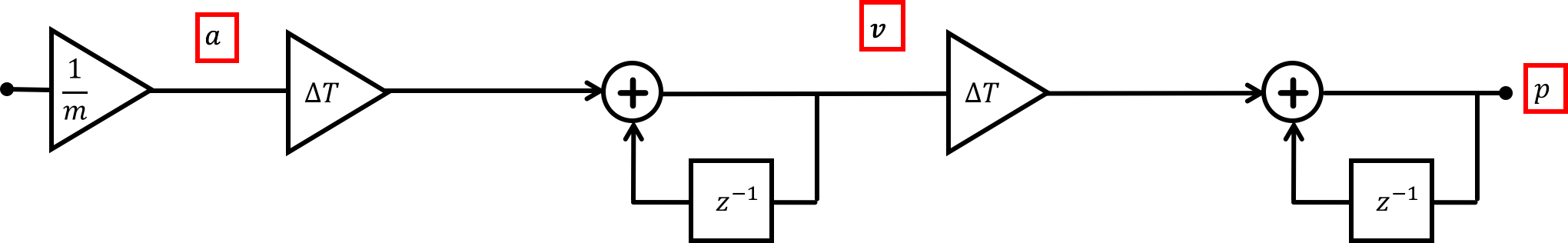
These states will be held by the following six variables (three for each axis, with one for acceleration, one for velocity, and one for position) and we are making them global right now.
float x_pos; //x pos state
float y_pos; //y pos state
float x_vel; //x vel state
float y_vel; //y pos state
float x_accel; //x accel state
float y_accel; //y accel state
3) moveBall
It is now your job to write function called moveBall that updates the position state of the ball based on current velocity and previous position. Use the system diagrams drawn out above as well as what we learned when discussing difference equations in the discrete time part of this week's exercises to determine what should go into moveBall. First just get moveBall to properly integrate velocity with position. Submit that working version into the checker below to make sure you're on the right track. Don't forget to scale time appropriately!!
3.1) moveBall v1
Submit a moveBall implementation that does ONLY the velocity to position integration! You have access to all the global variables in the starter code. For now, do NOT take into account the boundaries of the screen.

When you pass the check, add this working function into the code skeleton, upload and see what happens. It will be awesome for a second...and then sadness...and then not sadness....and then sadness again...the ball should appear to be teleporting from one side of the screen to the other after flying across.
3.2) moveBall v2
What happened? Well our physics engine worked well, but we never bothered to code up wall collissions. So you just simulated yourself right off the edge of the screen which is no good. Now you need to make an even better version ofmoveBall that handles wall collissions.
This new better moveBall method should also handle wall collisions in a completely elastic manner meaning that the normal velocity is perfectly negated as shown in the figure below when a wall is encountered:
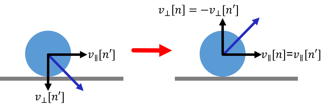
We can describe this operation as:
Test your code out locally and be sure to paste in a fully functioning (from the previous section) in order to get everything working correctly! When you feel like your code is good, paste it in below for checking/grading purposes. Paste only the moveBall method in below. We will test it by dropping it into a simulated game in our code.
YOU MUST fully reflect the velocity with this ball. Be very careful with x_pos and y_pos during a bounce.
For example, let's say the ball is a single pixel at (32,158) and is moving 3 pixels in the +y direction per time step (really large) and it cannot move beyond y=159 (i.e. BOTTOM_LIMIT is 159). At the next time step it must be at (32,157) because it moved down +1 pixel towards the wall, then -2 pixel away from the wall (for full 3 pixel reflection)
Do NOT hardcode the boundary values (0, 63, 127, or whatever). Instead use LEFT_LIMIT, RIGHT_LIMIT, etc.
When you have passed the tutor check above, you should have a really nice perpetual motion machine of a rolling ball. This is cool, but we're going to use this in game development in the future and this might cause some issues (in something like pong it wouldn't, but in a simulated soccer or billiards game it would). So what's happening? The answer is that our physics model right now has no loss mechanism. The ball is initially accelerated and it bounces around a bunch, but it never loses any of the simulated kinetic energy imparted on it at the start of the simulation. An energy loss mechanism such as friction or non-ideal elastic collisions with walls will make the system more realistic. So let's do that. Let's pull some energy out of our system (and make it "lossy") by adding in dynamic friction. In general friction manifests as a force in the opposite direction of the velocity
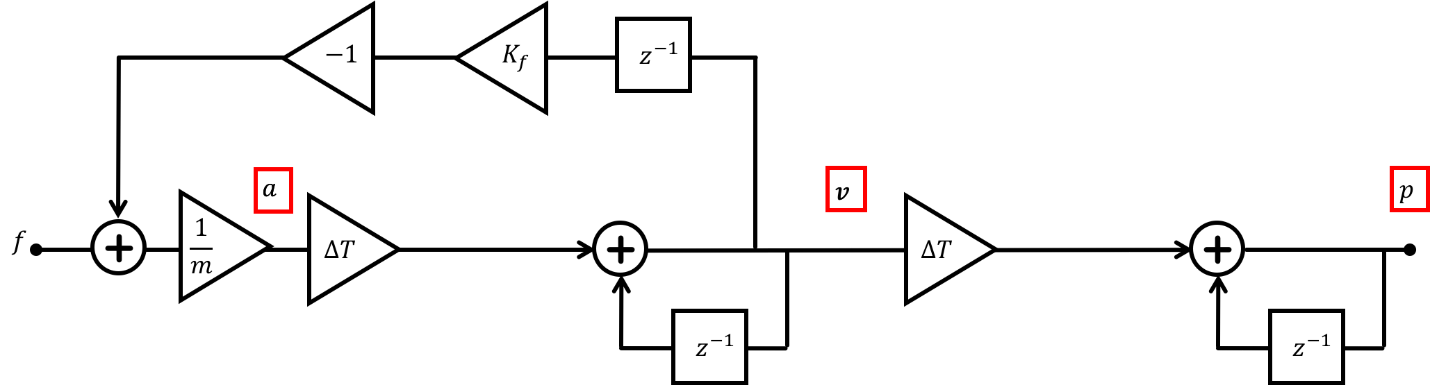
We can implement this mechanism by changing our system block diagram. A modified system diagram for this new simulation is shown below. Notice how the location where the velocity state exists is now also "fed back", multiplied by the friction coefficient, and then subtracted from the force being applied by gravity. The subtraction part is necessary to account for the fact that the force exerted by dynamic friction is opposing the sign of the velocity.
We also want to add a lossy bounce characteristic. Where before 100% of normal velocity would reflect upon collision with a wall in real life that will never happen...in the case of a rubber ball bouncing off a wall, the compression and then expansion of the rubber is not 100% efficient...instead some of that energy is given off as heat, sound, enjoyment, etc... So we're going to now have some loss, which will be represented by the following:
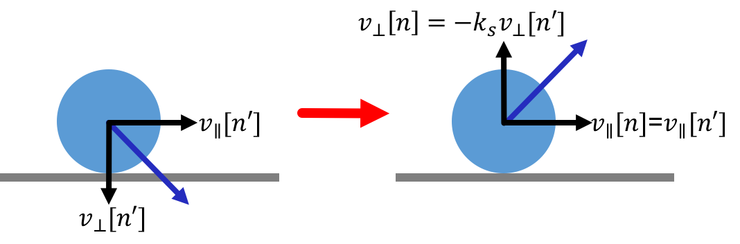
You can assume two additional variables are defined and should be included in the code: K_SPRING is a float that represents the spring coefficient of the ball and K_FRICTION is a float that represents the friction coefficient.
3.3) step v2
Modify the step and moveBall functions so that they now take into account friction. With wall bounces, be particularly careful with x_pos and y_pos. Remember that K_SPRING will decrease the distance of a wall bounce. From the previous example, we had a ball at (32,158), which was trying to move 3 units in the +y direcion. We had BOTTOM_LIMIT = 159. Let's now say K_SPRING is 0.5. The ball will move +1 unit, hit the wall, and then move -2 * 0.5 = -1 unit back off the wall, ending at (32,158). Here, the inelastic collision has decreased the "bounce back" distance from 2 units in the -y direction to 1 unit in the -y direction.
In the box below implement an improved version of step only! (you'll implement an new version of moveBall in the next section.)
3.3.1) moveBall v3
Now implement an improved version of moveBall
Once you've got these two bits of code, put them on your microcontroller and enjoy a bouncing ball. It should jump approximately every time you push your button! If it doesn't make sure you switch is hooked up, and that you have the right versions of the code in your file! Feel free to change friction or the initial "kick" in the setup to get different behaviors! We'll build on some of this ball physics in future exercises.
Footnotes
1Pin 19 is turning out to be buggy since it shares some internal resources with the I2C bus and the WiFi