If you are a current student, please Log In for full access to the web site.
Note that this link will take you to an external site (https://shimmer.csail.mit.edu) to authenticate, and then you will be redirected back to this page.
1) Discrete Time Signals and Systems
In Week 1 we built a system or two that responded to inputs in various ways. In particular our input was a button. While we may not have been thinking specifically about it at the time, the system we were designing did not work and respond __continuously__ in time, but rather in discrete steps. Even though our microcontroller is running so fast that it is hard to recognize it as a human, it is really running through its life doing one step and then another and then another...As mentioned previously, our standard ESP32 code has a structure like:
void setup(){
  //runs once
}

void loop(){
    //runs repeatedly

}
If we're not doing much inside our loop function, it can run extremely fast, but depending on how fast it is running and how fast the outside events it is interacting with happen, it **may** or **may not** be sufficient to just assume it runs "really fast". This has really profound implications in how we handle this data. While in physics and calculus you've probably been taught to model systems using the continuous-time variable $t$ and to treat things like derivatives and integrals from the perspective of continuous time, in most modern digital systems (including our own), this appraoch doesn't work.
Consider a situation where you have a light sensor connected to your microcontroller and you are capable of getting measurements from it by doing analogRead calls to the correct pin. (Analog readings provide back values that can be one of many values in a range, as opposed to the digital readings we dealt with in Lab 01A and B). Let's say you were building a tanning booth and wanted to make sure you didn't get too much light exposure. You could integrate over time the level of the light signal and that could give you a good idea of the total "exposure" to the light. Mathematically the exposure E(t) at some point in time t_1 could be calculated doing the following if we have a light signal, l(t):
This is pretty standard calculus so this should not be blowing anyone's mind...but how would you actually implement an integral on a microcontroller? We can't just draw the integral squiggle in code and have it do that. Furthermore, if you don't know what your light signal is going to be ahead of time (it is not some nice and easy function like l(t) = 1.23t), and you have to figure out the signal as you are making measurements, what do you do? Solving for the definite integral only makes sense when you know the function you have, but if your function isn't known, it seems we might have a problem. On top of all of this, we have the issue that our signal doesn't "exist" in continuous time. Our microcontroller will really only see the signals in disticnt samples over time similar to what is shown below where the loop takes 4 milliseconds to run.
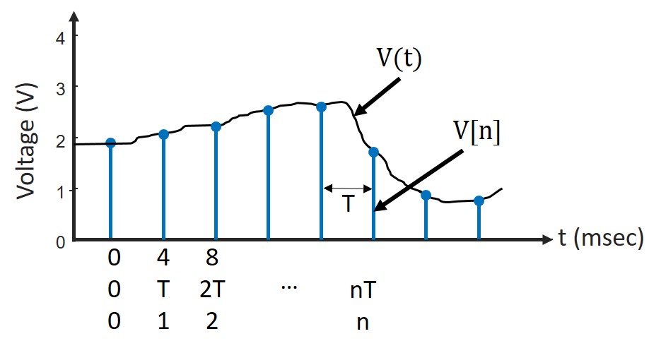
This means that from the perspective of our microcontroller, our signal isn't continous since it is only catching discontinuous samples of it. In order to fix this problem, we need to think about our signals in terms of time steps (or number of iterations through the loop), which we usually express with the variable n. Now the universe really does run in continuous time, so there is an actual relationship between continuous and discrete time. In particular:
uint32_t time_counter; //always positive so no need to worry about it being signed
const uint32_t DT = 50; //sample period (milliseconds)

void setup(){
  Serial.begin(115200);
  time_counter = millis();
}

void loop(){
  int value = analogRead(A5);
  Serial.println(value);
  while (millis() - time_counter < DT); //wait and do nothing
  time_counter = millis(); //update time_counter to newest time
}
In this code, we're taking a measurement from analog pin 5 (A5), printing it up via the Serial port and then waiting until a certain number of milliseconds have passed by surpasses dt, which is our sample period before continuing on (and restarting the loop). Doing it this way ensures our loop runs at a continuous rate.
We use square brackets to represent the time variable of signals in discrete time. As a result, if we assume the system starts when t=0, the discrete time value v[5] will equal the value of the continuous time signal v(t) at 5\cdot 0.05\text{ seconds} or v(0.25).
This may seem like a weird way to think about the world, but it is very powerful for producing responses to signals in code, and for when you need to start thinking about concepts like integration or differentiation and how code can progress in time.
1.1) Representations
We're usually going to represent our discrete-time systems in ways very similar to continuous-time systems. We call these types of equations difference equations, and it is important to remember that their domain is only for integer values of n (it is meaningless to analyze a difference equation at fraction value of n like 1.5 or something). This is because your microcontroller only knows what the signal value is at the moment it is sampled. In between those sample times, it doesn't have any idea. Let's take a look at the simple difference equation below:Here we're saying that the variable y is equal to the product of some constant k and some variable x. Very importantly, it is specifying timesteps too! A more refined way of saying this would be the value of y at a given time step is equal to the product of constant k and the value of x at that same time step.
We can write out difference equations using block diagrams to better visualize the flow of information and signals. We can represent this in diagram form with the following:

In the diagram, we read from left-to-right, as we do when reading code or most text. The variable x is our input and y is our output. The triangle represents a gain block which simply multiplies the input by a constant to generate the output.
A code implementation of this system in our ESP32 C++ environment would look like the following:
uint32_t time_counter;
uint32_t DT = 50; //sample period (milliseconds)
void setup(){
  Serial.begin(115200);
  time_counter = millis();
}

void loop(){
  float k = 4; //some constant
  float x = analogRead(A3);
  float y = k*x;
  Serial.println(y);
  while (millis() - time_counter < DT); //wait and do nothing
  //in C++ you don't need {} in your while loop if you do nothing in them
  //or if they are one line long
  time_counter = millis(); //update time_counter to newest time
}
Basically every time (time step) through the loop y is calculated to be based off of the current value of x (here based on some sensor reading we're assuming is attached to analog pin 3) multiplied by a constant k.
1.2) Delays in Time
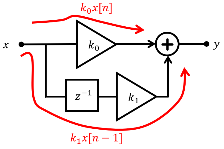
OK, maybe we want y to be based not only what x currently is, but a previous value of x. This is where the [n] part of the variables really comes into play. n is our time-step variable, which oftentimes in our code will be equivalent to the number of times through a loop (either the mainloop function or possibly a smaller loop you wrote, like a for loop). If we wanted y to be based on the current value of x multiplied by a constant k_0 and the previous value of x multiplied by a constant k_1, we would express that using the following difference equation:
Here the n-1 refers to the value of x on the previous timestep or iteration through the loop function. Diagrammatically this would look like the following:
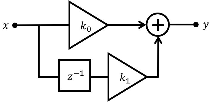
There are two new symbols from the previous simpler system. The first is the circle with a plus symbol which is the addition operator. Signal lines going into the adder are denoted with arrows. The second is a delay operator which we indicated by the letter z raised to the -1th power. The meaning of the z is really a topic for another class (or you can ask in office hours or on Piazza or look up z-transforms on Wikipedia). What matters for us now is that the order of the negative exponent indicates how many steps of delay are in place. If the delay box had a z^{-5} in it that would imply there is a delay of 5 time steps for a signal going through it. That doesn't mean that nothing comes out of the delay block for five time steps...it only means that the signal coming out of the delay block at some timestep m was fed into the input of that block at timestep m-5 or five time steps in the past:
Programmatically if we wanted to write up such a system from above in C/C++ it could look like:
uint32_t time_counter;
uint32_t DT = 50; //sample period (milliseconds)
float x_old = 0;  //global variable that must have scope outside the loop.
void setup(){
  Serial.begin(115200);
  time_counter = millis();
}

void loop(){
  float k0 = 5; //first constant
  float k1 = 3.2; //second constant
  float x_current = analogRead(A3);
  float y = k0*x_current + k1*x_old;
  x_old = x_current; // Hand off x to "storage variable" for use next time through the loop.
  Serial.println(y);
  while (millis() - time_counter < DT); //wait and do nothing
  time_counter = millis(); //update time_counter to newest time
}
A few important takeaways from this bit of code. In the first example with no delays in time (no n-1) you should see that there was no need for global variables (variables that lived beyond each iteration of the loop.) Previously we declared new variables each time through and then those variables were destroyed every time the loop function completed an iteration. Here, however, the system can no longer "live in the moment" and needs some way of remembering previous values. This is accomplished by saving a value at the end of the loop (saying x_old = x_current). By doing this we are able to access an older value from a previous iteration of the loop and use it as needed.
1.3) Averaging Filtering
OK, so now that we've got a little bit of discrete time and difference equations in our heads we could ask, so what? What can we do with them? We can make a averager, which we'll find lots of uses for this semester. Averaging will tend to keep only the "persistent" part of a signal. This is often what we're interested in, i.e., filtering out random blips that may be mixed in.
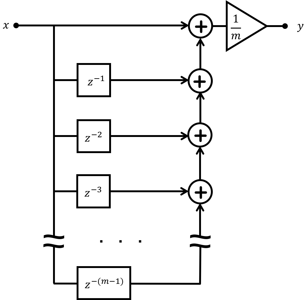
A filter that "moves" along with the data as it is fed in, averaging the m last samples is known as a moving-average filter. In difference equation form we can create a three-sample moving-average filter with the following equation:
This equation is saying that the value of y (our output from this filter) at any given time step is going to be based on the three-way moving average of what x is at that timestep [n], one timestep prior [n-1] and two timesteps prior [n-2]. This should look familiar to you from when you've done averaging before. The only new parts are that we're working in discrete time steps!
In code this would look like:
uint32_t time_counter;
uint32_t DT = 50; //sample period (milliseconds)

float x_older = 0; //used to store n-1 value
float x_oldest = 0; //used to store n-2 value
void setup(){
  Serial.begin(115200);
  time_counter = millis();
}

void loop(){
  float x_current = analogRead(A3);
  float y = 1.0/3.0*x_current + 1.0/3.0*x_older + 1.0/3.0*x_oldest;
  Serial.println(y);
  x_oldest = x_older;
  x_older = x_current;
  while (millis() - time_counter < DT); //wait and do nothing
  time_counter = millis(); //update time_counter to newest time
}
You can see that we need two global variables to exist outside the "scope" of the loop function in order to remember the values, and that we reassign them at the end of every loop iteration.
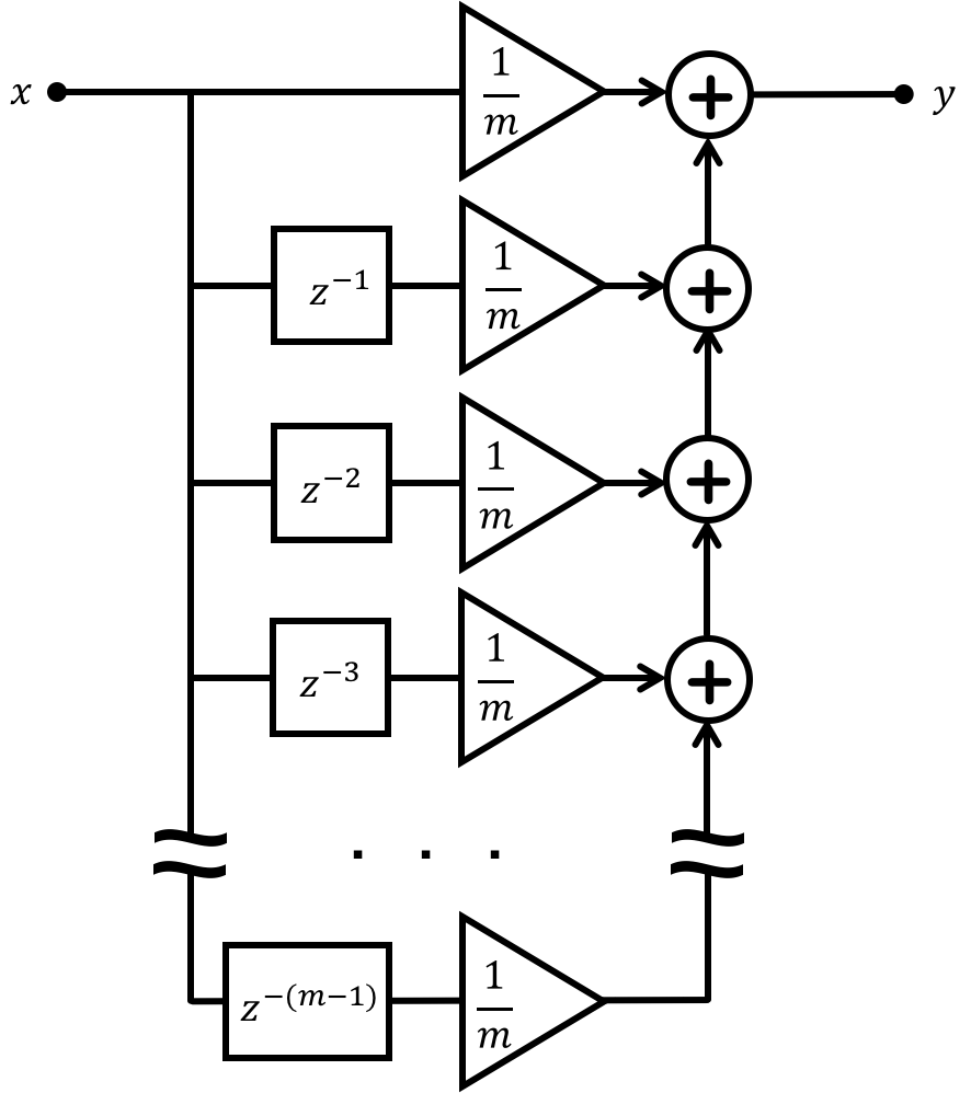
We don't need to only pick 3 timesteps either...in fact we could do an arbitrary number m for a m-way moving average filter and express that as:
which we can represent in a diagram as follows:
We can also pull out factors in difference equations, just like we can do in continuous-time equations, so we can also get this:
which would look like this in diagram form:
Code-wise that would involve change this line:
float y = 1.0/3.0*x_current + 1.0/3.0*x_older + 1.0/3.0*x_oldest;
to the following:
float y = 1.0/3.0*(x_current + x_older + x_oldest);
2) Back to Difference Equations
You can also change what all the gain blocks are for each delayed path
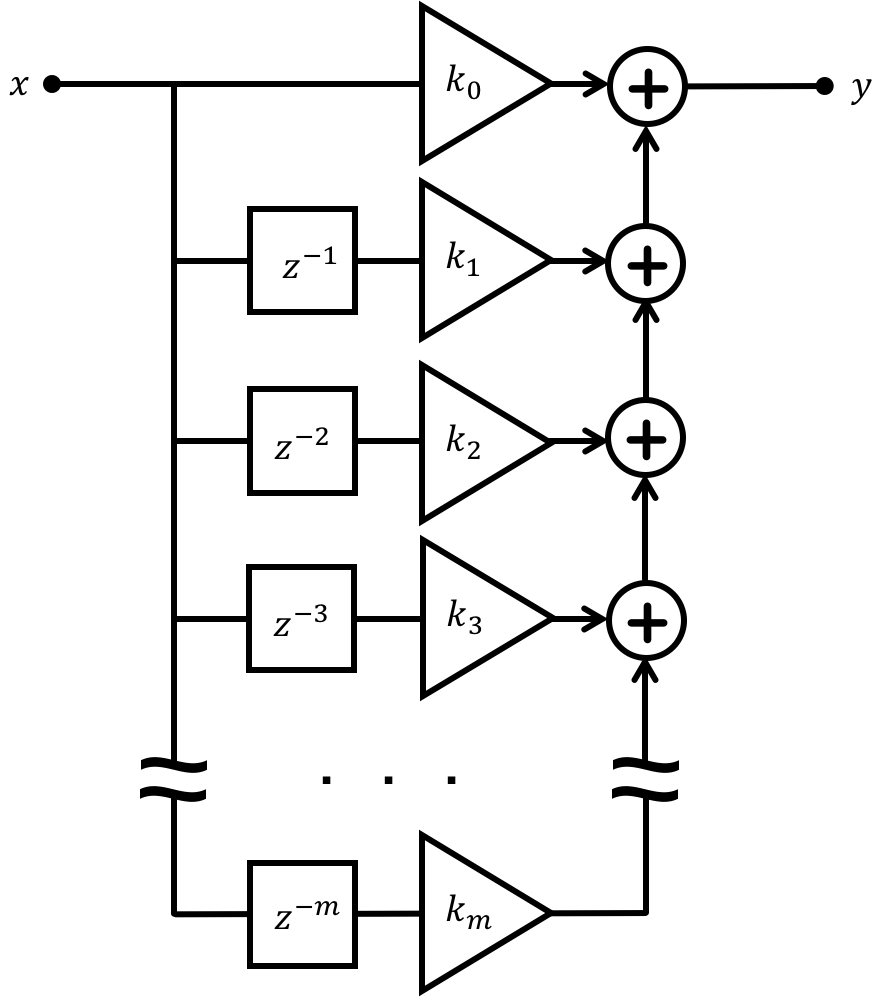
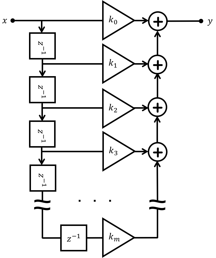
While we won't go into the derivations in this class since it would take too long to set up the math, you can actually engineer these k coefficients to give really complex filtering such as removing bass or treble in audio filtering and many other things. We call this general type of filter a Finite Impulse Response filter (FIR), and that averaging filter you just made is a restricted type of that. Noise-canceling headphones will often make use of FIR filters to dynamically filter out unwanted signals. In real-life, FIR filters can be thousands of values long (going back to like x[n-1000] is not rare).
2.1) Feedback
So we just said that we can classify the type of filters as Finite Impulse Response filter. What this basically means is that if you give a bit of signal to the input of the system, it will eventually forget that input which should make sense since it only remembers so many timesteps into the past. This should make sense if we think about our original hard-coded second order code above on this page. The information cycles through the global variables until it is eventually forgotten.
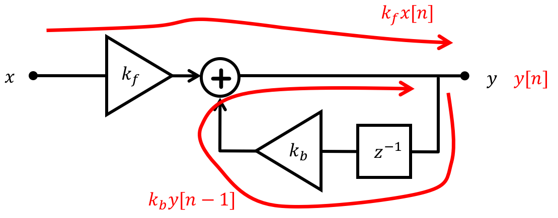
This raises the question, however, that if there is an FIR, is there something called an IIR...an Infinite Impulse Response filter, which would be something that never forgets an input signal? There is indeed, and we get this from what is called feedback and occurs when a variable's value on a given timestep is based directly upon one or several values of that variable on previous timestep(s). Consider the following difference equation:
which diagramatically can be represented as the following:
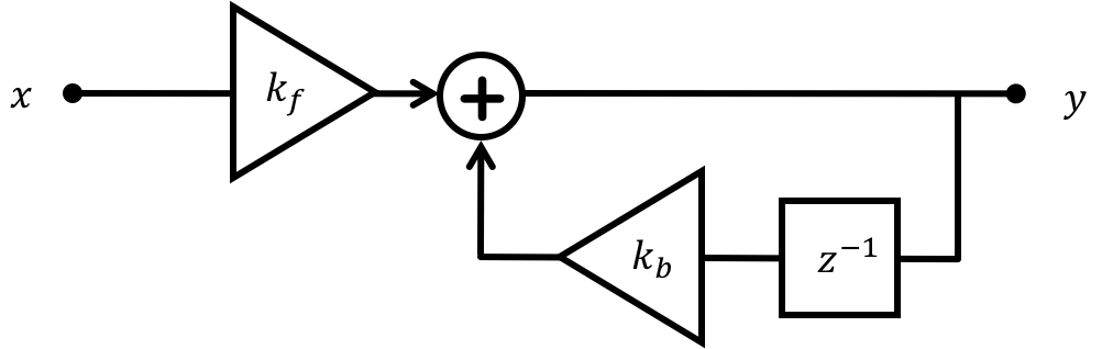
Note that an arrow/signal path is going backwards in the block diagram! This is indicative of feedback. In this case, y is based on its value from the previous time step as well as the input value from x like before.
In code, feedback takes the following form:
uint32_t time_counter;
uint32_t DT = 50; // Sample period (milliseconds)
int y = 0;

void setup(){
  Serial.begin(115200);
  time_counter = millis();
}

void loop() {
  y  = y + analogRead(A3);	// new y is equal to old y plus the input
  Serial.println(y);
  while (millis() - time_counter <DT); // Wait and do nothing
  time_counter = millis(); // Reset to 0 for next count up
}
Because of how the assignment (=) operator works in most programming languages, where the right half is evaluated before the left half the line of code:
y = y + analogRead(A3);
is just like
analogRead(A3) and y = y.
We can also have multiple feedback paths as indicated below:
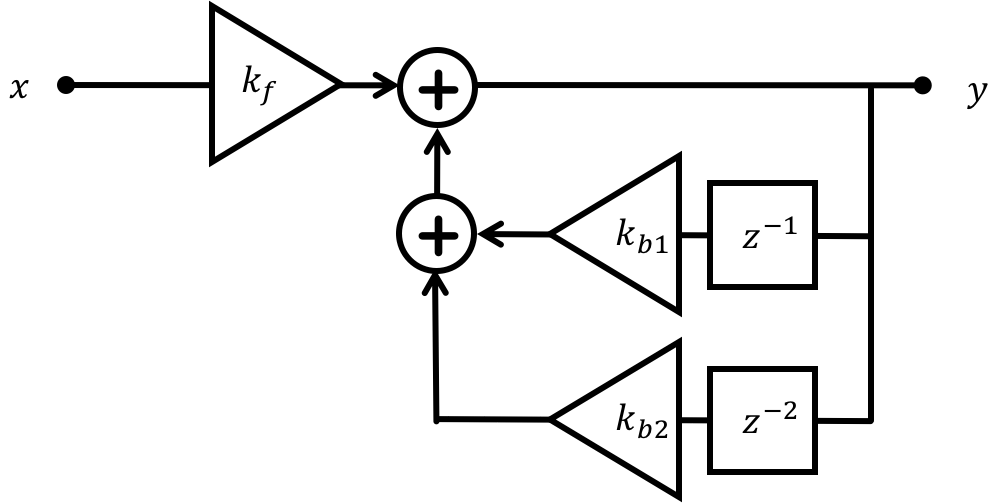
which would have a difference equation of:
More generally, we can write any difference equation of the type we have been discussing (linear, with constant coefficients) that has both feedback (IIR) terms and feedforward (FIR) terms in the form:
2.2) Example
Given this formulation, what would the difference equation for the system below look like? Enter the input and output coefficients, called dCoeffs and cCoeffs, respectively, in the form of a Python list below:
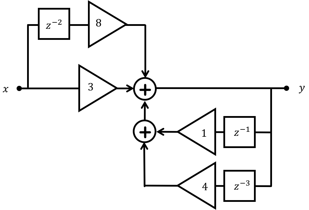
Difference Equation:
cCoeffs (output):
The coefficients currently entered represent the following difference equation:
$$y[n] = 0$$

Now write a C++ implementation of this system. The system is comprised of two parts:
float vals[6]: An already-defined global array which will start filled with 0's and which should be updated over time to store past values.float system(float x);: A function that we can call (and that you write) which repeatedly that takes in an inputfloat xand returns the output. Each time we call the function, it is equivalent to a new timestep.
The function should utilize the array to hold values at a global level. It is up to you to decide how to use the array. The first two test cases in particular are the system's outputs in response to very simple inputs so use those in particular to debug.
2.3) Discrete Time Integration
Now let's return to our original problem how do we do integration in our discrete time system? The answer, is a discrete time integrator.
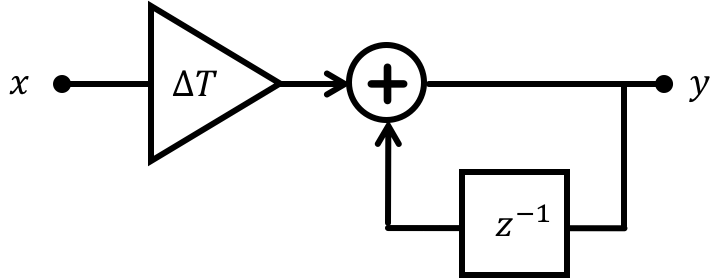
With difference equation of:
This should make some intuitive sense, and is oftentimes how people first learn the idea behind integrals. This system is saying that if y is the integral in time of x then y should be whatever it was previously (y[n-1]) plus whatever x is now multiplied by the time step duration \Delta T over which that input is assumed to have been valid. We're definitely making an assumption with this (that x will stay the same during the upcoming interval and there's a whole lot to study in terms of what happens during that interval and how valid that assummption is), but for many purposes this is a valid approach to discrete-time integration.
Write a discrete time integrator below that uses a already-defined global variable float total; that is initialized to 0 and should contain the integration amount. The function when called will also have access to an already-defined variable representing \Delta T (in seconds) called const float Delta_T;. Upon being given an input, the function should return the current output of its integration. Ideally the function is designed to work in a situation where it is called every \Delta T seconds by an outer piece of code (that way the integration makes sense).